sfepy.solvers.ts_solvers module
Time stepping solvers.
- class sfepy.solvers.ts_solvers.AdaptiveTimeSteppingSolver(conf, nls=None, context=None, **kwargs)[source]
Implicit time stepping solver with an adaptive time step.
Either the built-in or user supplied function can be used to adapt the time step.
Kind: ‘ts.adaptive’
For common configuration parameters, see
Solver.Specific configuration parameters:
- Parameters:
- t0float (default: 0.0)
The initial time.
- t1float (default: 1.0)
The final time.
- dtfloat
The time step. Used if n_step is not given.
- n_stepint (default: 10)
The number of time steps. Has precedence over dt.
- quasistaticbool (default: False)
If True, assume a quasistatic time-stepping. Then the non-linear solver is invoked also for the initial time.
- adapt_funcallable(ts, status, adt, context, verbose)
If given, use this function to set the time step in ts. The function return value is a bool - if True, the adaptivity loop should stop. The other parameters below are collected in adt, status is the nonlinear solver status, context is a user-defined context and verbose is a verbosity flag. Solvers created by
Problemuse the Problem instance as the context.- dt_red_factorfloat (default: 0.2)
The time step reduction factor.
- dt_red_maxfloat (default: 0.001)
The maximum time step reduction factor.
- dt_inc_factorfloat (default: 1.25)
The time step increase factor.
- dt_inc_on_iterint (default: 4)
Increase the time step if the nonlinear solver converged in less than this amount of iterations for dt_inc_wait consecutive time steps.
- dt_inc_waitint (default: 5)
The number of consecutive time steps, see dt_inc_on_iter.
- name = 'ts.adaptive'
- class sfepy.solvers.ts_solvers.BatheTS(conf, nls=None, context=None, **kwargs)[source]
Solve elastodynamics problems by the Bathe method.
The method was introduced in [1].
[1] Klaus-Juergen Bathe, Conserving energy and momentum in nonlinear dynamics: A simple implicit time integration scheme, Computers & Structures, Volume 85, Issues 7-8, 2007, Pages 437-445, ISSN 0045-7949, https://doi.org/10.1016/j.compstruc.2006.09.004.
Kind: ‘ts.bathe’
For common configuration parameters, see
Solver.Specific configuration parameters:
- Parameters:
- t0float (default: 0.0)
The initial time.
- t1float (default: 1.0)
The final time.
- dtfloat
The time step. Used if n_step is not given.
- n_stepint (default: 10)
The number of time steps. Has precedence over dt.
- is_linearbool (default: False)
If True, the problem is considered to be linear.
- has_time_derivativesbool (default: False)
If True, the problem equations contain time derivatives of other variables besides displacements. In that case the cached constant matrices must be cleared on time step changes.
- var_namesdict
The mapping of variables with keys ‘u’, ‘du’, ‘ddu’ and ‘extra’, and values corresponding to the names of the actual variables. See var_names returned from
transform_equations_ed()
- create_nlst2(nls, dt, u0, u1, v0, v1)[source]
The second sub-step: the three-point Euler backward method.
- name = 'ts.bathe'
- class sfepy.solvers.ts_solvers.CentralDifferenceTS(conf, nls=None, tsc=None, context=None, **kwargs)[source]
Solve elastodynamics problems by the explicit central difference method.
It is the same method as obtained by using
NewmarkTSwith ,
,  , but uses a simpler code.
It is also mathematically equivalent to the
VelocityVerletTSmethod. The current implementation code is essentially the same.This solver supports, when used with
RMMSolver, the reciprocal mass matrix algorithm, seeMassTerm.Kind: ‘ts.central_difference’
For common configuration parameters, see
Solver.Specific configuration parameters:
- Parameters:
- t0float (default: 0.0)
The initial time.
- t1float (default: 1.0)
The final time.
- dtfloat
The time step. Used if n_step is not given.
- n_stepint (default: 10)
The number of time steps. Has precedence over dt.
- is_linearbool (default: False)
If True, the problem is considered to be linear.
- has_time_derivativesbool (default: False)
If True, the problem equations contain time derivatives of other variables besides displacements. In that case the cached constant matrices must be cleared on time step changes.
- var_namesdict
The mapping of variables with keys ‘u’, ‘du’, ‘ddu’ and ‘extra’, and values corresponding to the names of the actual variables. See var_names returned from
transform_equations_ed()
- name = 'ts.central_difference'
- class sfepy.solvers.ts_solvers.ElastodynamicsBaseTS(conf, nls=None, tsc=None, context=None, **kwargs)[source]
Base class for elastodynamics solvers.
Assumes block-diagonal matrix in u, v, a.
- class sfepy.solvers.ts_solvers.GeneralizedAlphaTS(conf, nls=None, tsc=None, context=None, **kwargs)[source]
Solve elastodynamics problems by the generalized
 method.
The method was introduced in [1].
The method is unconditionally stable provided
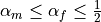 ,
, 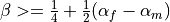 .
.The method is second-order accurate provided
 . This is used when gamma is
 None.High frequency dissipation is maximized for
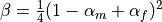 . This is used when beta is
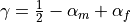
 None.The default values of
 ,
,  (if alpha_m or
alpha_f are
(if alpha_m or
alpha_f are None) are based on the user specified high-frequency dissipation parameter rho_inf.
Special settings:
 corresponds to the HHT- method.
 corresponds to the WBZ- method.
- , produces the Newmark method.
[1] J. Chung, G.M.Hubert. “A Time Integration Algorithm for Structural Dynamics with Improved Numerical Dissipation: The Generalized-
Method” ASME Journal of Applied Mechanics, 60,
371:375, 1993.Kind: ‘ts.generalized_alpha’
For common configuration parameters, see
Solver.Specific configuration parameters:
- Parameters:
- rho_inffloat (default: 0.5)
The spectral radius in the high frequency limit (user specified high-frequency dissipation) in [0, 1]: 1 = no dissipation, 0 = asymptotic annihilation.
- alpha_mfloat
The parameter
.- alpha_ffloat
The parameter
.- betafloat
The Newmark-like parameter
 .
.- gammafloat
The Newmark-like parameter
 .
.- t0float (default: 0.0)
The initial time.
- t1float (default: 1.0)
The final time.
- dtfloat
The time step. Used if n_step is not given.
- n_stepint (default: 10)
The number of time steps. Has precedence over dt.
- is_linearbool (default: False)
If True, the problem is considered to be linear.
- has_time_derivativesbool (default: False)
If True, the problem equations contain time derivatives of other variables besides displacements. In that case the cached constant matrices must be cleared on time step changes.
- var_namesdict
The mapping of variables with keys ‘u’, ‘du’, ‘ddu’ and ‘extra’, and values corresponding to the names of the actual variables. See var_names returned from
transform_equations_ed()
- name = 'ts.generalized_alpha'
- class sfepy.solvers.ts_solvers.NewmarkTS(conf, nls=None, tsc=None, context=None, **kwargs)[source]
Solve elastodynamics problems by the Newmark method.
The method was introduced in [1]. Common settings [2]:
name
kind
beta
gamma
Omega_crit
trapezoidal rule:
implicit
1/4
1/2
unconditional
linear acceleration:
implicit
1/6
1/2

Fox-Goodwin:
implicit
1/12
1/2

central difference:
explicit
0
1/2
2
All of these methods are 2-order of accuracy.
[1] Newmark, N. M. (1959) A method of computation for structural dynamics. Journal of Engineering Mechanics, ASCE, 85 (EM3) 67-94.
[2] Arnaud Delaplace, David Ryckelynck: Solvers for Computational Mechanics
Kind: ‘ts.newmark’
For common configuration parameters, see
Solver.Specific configuration parameters:
- Parameters:
- betafloat (default: 0.25)
The Newmark method parameter beta.
- gammafloat (default: 0.5)
The Newmark method parameter gamma.
- t0float (default: 0.0)
The initial time.
- t1float (default: 1.0)
The final time.
- dtfloat
The time step. Used if n_step is not given.
- n_stepint (default: 10)
The number of time steps. Has precedence over dt.
- is_linearbool (default: False)
If True, the problem is considered to be linear.
- has_time_derivativesbool (default: False)
If True, the problem equations contain time derivatives of other variables besides displacements. In that case the cached constant matrices must be cleared on time step changes.
- var_namesdict
The mapping of variables with keys ‘u’, ‘du’, ‘ddu’ and ‘extra’, and values corresponding to the names of the actual variables. See var_names returned from
transform_equations_ed()
- extra_variables = True
- name = 'ts.newmark'
- class sfepy.solvers.ts_solvers.SimpleTimeSteppingSolver(conf, nls=None, context=None, **kwargs)[source]
Implicit time stepping solver with a fixed time step.
Kind: ‘ts.simple’
For common configuration parameters, see
Solver.Specific configuration parameters:
- Parameters:
- t0float (default: 0.0)
The initial time.
- t1float (default: 1.0)
The final time.
- dtfloat
The time step. Used if n_step is not given.
- n_stepint (default: 10)
The number of time steps. Has precedence over dt.
- quasistaticbool (default: False)
If True, assume a quasistatic time-stepping. Then the non-linear solver is invoked also for the initial time.
- name = 'ts.simple'
- class sfepy.solvers.ts_solvers.StationarySolver(conf, nls=None, context=None, **kwargs)[source]
Solver for stationary problems without time stepping.
This class is provided to have a unified interface of the time stepping solvers also for stationary problems.
Kind: ‘ts.stationary’
For common configuration parameters, see
Solver.Specific configuration parameters:
- Parameters:
- name = 'ts.stationary'
- class sfepy.solvers.ts_solvers.VelocityVerletTS(conf, nls=None, tsc=None, context=None, **kwargs)[source]
Solve elastodynamics problems by the explicit velocity-Verlet method.
The algorithm can be found in [1].
It is mathematically equivalent to the
CentralDifferenceTSmethod. The current implementation code is essentially the same, as the mid-time velocities are not used for anything other than computing the new time velocities.[1]Swope, William C.; H. C. Andersen; P. H. Berens; K. R. Wilson (1 January 1982). “A computer simulation method for the calculation of equilibrium constants for the formation of physical clusters of molecules: Application to small water clusters”. The Journal of Chemical Physics. 76 (1): 648 (Appendix). doi:10.1063/1.442716
Kind: ‘ts.velocity_verlet’
For common configuration parameters, see
Solver.Specific configuration parameters:
- Parameters:
- t0float (default: 0.0)
The initial time.
- t1float (default: 1.0)
The final time.
- dtfloat
The time step. Used if n_step is not given.
- n_stepint (default: 10)
The number of time steps. Has precedence over dt.
- is_linearbool (default: False)
If True, the problem is considered to be linear.
- has_time_derivativesbool (default: False)
If True, the problem equations contain time derivatives of other variables besides displacements. In that case the cached constant matrices must be cleared on time step changes.
- var_namesdict
The mapping of variables with keys ‘u’, ‘du’, ‘ddu’ and ‘extra’, and values corresponding to the names of the actual variables. See var_names returned from
transform_equations_ed()
- name = 'ts.velocity_verlet'
- sfepy.solvers.ts_solvers.adapt_time_step(ts, status, adt, context=None, verbose=False)[source]
Adapt the time step of ts according to the exit status of the nonlinear solver.
The time step dt is reduced, if the nonlinear solver did not converge. If it converged in less then a specified number of iterations for several time steps, the time step is increased. This is governed by the following parameters:
red_factor : time step reduction factor
red_max : maximum time step reduction factor
inc_factor : time step increase factor
inc_on_iter : increase time step if the nonlinear solver converged in less than this amount of iterations…
inc_wait : …for this number of consecutive time steps
- Parameters:
- tsVariableTimeStepper instance
The time stepper.
- statusIndexedStruct instance
The nonlinear solver exit status.
- adtStruct instance
The object with the adaptivity parameters of the time-stepping solver such as red_factor (see above) as attributes.
- contextobject, optional
The context can be used in user-defined adaptivity functions. Not used here.
- Returns:
- is_breakbool
If True, the adaptivity loop should stop.
- sfepy.solvers.ts_solvers.gen_multi_vec_packing(di, names, extra_variables=False)[source]
Return DOF vector (un)packing functions for nlst. For multiphysical problems (non-empty ie slice for extra variables) the unpack() function accepts an additional argument mode that can be set to ‘full’ or ‘nls’.
The following DOF ordering must be obeyed:
The full DOF vector:
---iue---|-iv-|-ia--iu-|-ie-|
- sfepy.solvers.ts_solvers.standard_ts_call(call)[source]
Decorator handling argument preparation and timing for time-stepping solvers.
- sfepy.solvers.ts_solvers.transform_equations_ed(equations, materials)[source]
Transform equations and variables for
ElastodynamicsBaseTS-based time stepping solvers. The displacement variable name is automatically detected by seeking the second time derivative, i.e. the ‘dd’ prefix in variable names.