User’s Guide

Gensei is a software for generating serial sections through objects with known statistical properties and simulating stereological quantification in 3D.

Introduction

The purpose of gensei is to have a simple, open source tool to generate images of slices of a volume filled with objects (e.g. ellipsoids) with known statistical and other properties (e.g. total volume, volume fractions, number of objects), to verify information obtained by the stereological methods.

Stereology

Modern stereological methods are used for quantitative and qualitative description of objects, such as metals, stones, biological tissues, and their components. The stereology was defined by Weibel (1981) as “a body of mathematical methods relating three-dimensional measurements obtainable on sections of the structure”. The principles of stereology have one common feature: They make use of random tissue sections of negligible thickness, on which a test system is placed at random. This test system is made up of probes in the form of points, lines, or planar areas, depending on the information sought, see Weibel (1966).

The earlier decade of application of stereological methods on biological specimens (liver cells, muscles, and other systems) is described in Weibel (1966, 1981). From its beginning the stereology reached a great advancement and presently belongs to the most used methods for unbiased quantification of number, length, surface area and volume of specimen attributes of samples of various sizes and structures in the fields of biology, metallography, and petrography and may reveal important information about the function and organization of the parts being studied (organs, tissues, grains, etc.).

The stereological techniques are in detail described in following works: Gundersen and Jensen (1987), Gundersen et al. (1988a), Gundersen et al. (1988b), Howard and Reed (1998), Mandarim-de-Lacerda (2003), Mouton (2001), Nyengaard (1999), Nyengaard and Gundersen (2006), Russ and Dehoff (1999).

References

Gundersen and Jensen (1987): Gundersen, H. J. G. and Jensen, E. B. (1987). The efficiency of systematic sampling in stereology and its prediction. Journal of Microscopy, 147:229-263. (http://www.ncbi.nlm.nih.gov/pubmed/3430576)

Gundersen et al. (1988a): Gundersen, H. J. G., Bendtsen, T. F., Korbo, L., Marcussen, N., Møller, A., Nielsen, K., Nyengaard, J. R., Pakkenberg, B., Sørensen, F. B., Vesterby, A., and West, M. J. (1988b). Some new, simple and efficient stereological methods and their use in pathological research and diagnosis. Acta Pathologica, Microbiologica et Immunologica Scandinavica, 96:379-394. (http://www.ncbi.nlm.nih.gov/pubmed/3288247)

Gundersen et al. (1988b): Gundersen, H. J. G., Bagger, P., Bendtsen, T. F., Evans, S. M., Korbo, L., Marcussen, N., Møller, A., Nielsen, K., Nyengaard, J. R., Pakkenberg, B., Sørensen, F. B., Vesterby, A., and West, M. J. (1988a). The new stereological tools: Disector, fractionator, nucleator and point sampled intercepts and their use in pathological research and diagnosis. Acta Pathologica, Microbiologica et Immunologica Scandinavica, 96:857-881. (http://www.ncbi.nlm.nih.gov/pubmed/3056461)

Howard and Reed (1998): Howard, C. V. and Reed, M. G. (1998). Unbiased Stereology: Three Dimensional Measurement in Microscopy. Royal Microscopical Society, Microscopy Handbook Series No. 41. Springer, New York.

Mandarim-de-Lacerda (2003): Mandarim-de-Lacerda, C. A. (2003). Stereological tools in biomedical research. Annals of the Brazilian Academy of Sciences, 75(4):469-486.(http://www.ncbi.nlm.nih.gov/pubmed/14605681)

Mouton (2001): Mouton, P. R. (2001). Principles and Practices of Unbiased Stereology: An Introduction for Bioscientists. The Johns Hopkins University Press, USA, Baltimore.

Nyengaard (1999): Nyengaard, J. R. (1999). Stereologic methods and their application in kidney research. Journal of the American Society of Nephrology, 10:1100-1123. (http://jasn.asnjournals.org/cgi/content/full/10/5/1100)

Nyengaard and Gundersen (2006): Nyengaard, J. R. and Gundersen, H. J. G. (2006). Sampling for stereology in lungs. European Respiratory Review, 15(101):107-114. (http://err.ersjournals.com/cgi/content/abstract/15/101/107)

Russ and Dehoff (1999): Russ, J. C. and Dehoff, R. T. (1999). Practical Stereology. Plenum Press, New York.

Weibel (1966): Weibel, E. R., Kistler, G. S., and Scherle,W. F. (1966). Practical stereological methods for morphometric cytology. The Journal of Cell Biology, 30:23-38. (http://www.ncbi.nlm.nih.gov/pubmed/5338131)

Weibel (1981): Weibel, E. R. (1981). Stereological methods in cell biology: Where are we - where are we going? The Journal of Histochemistry and Cytochemistry, 29(9):1043-1052. (http://www.jhc.org/cgi/reprint/29/9/1043)

Basic usage

The script volume_slicer.py can be used to place objects of known (given) geometrical and statistical properties into a (virtual) 3D box and then generate the slices. It can be called as:

Usage: volume_slicer.py [options] [filename]

If an input file is given, the object class options have no effect.

Default option values do _not_ override the input file options.


Options:
  --version             show program's version number and exit
  -h, --help            show this help message and exit
  -o filename           basename of output file(s) [default: ./slices/slice]
  -f format, --format=format
                        output file format (supported by the matplotlib
                        backend used) [default: png]
  -n int, --n-slice=int
                        number of slices to generate [default: 21]
  -d dims, --dims=dims  dimensions of specimen in units given by --units
                        [default: (10, 10, 10)]
  -u units, --units=units
                        length units to use [default: mm]
  -r resolution, --resolution=resolution
                        figure resolution [default: 600x600]
  --fraction=float      volume fraction of objects [default: 0.1]
  --fraction-reduction=float
                        volume fraction reduction factor [default: 0.9]
  --length-to-width=float
                        length-to-width ratio of objects [default: 8.0]
  --n-object=int        number of objects [default: 10]
  -t float, --timeout=float
                        timeout in seconds for attempts to place more
                        ellipsoids into the block [default: 5.0]
  --no-pauses           do not wait for a key press between fitting,
                        generation and slicing phases (= may overwrite
                        previous slices without telling!)

Further options can be set in an input file, see below.

Example input file

This file defines four classes of ellipsoids, the box and other necessary options.

# This is an example file with advanced settings. It can be called in ipython
# shell as: %run volume_slicer.py examples/myexample.py

#--------Settings of the properties of objects-----------
objects = {
    # objects of the first class
    'class 1' : {
        # geometry of the objects
        'kind' : 'ellipsoid',
        # color in RGB space, or one of
        # 'b'         blue
        # 'g'         green
        # 'r'         red
        # 'c'         cyan
        # 'm'         magenta
        # 'y'         yellow
        # 'w'         white
        'color' : 'r',
        # volume fraction of the objects of this class
        'fraction' : 0.2,
        # length-to-width ratio
        'length_to_width' : 8.0,
        # (0,1) allows to change the geometry of the objects when they can not
        # fit the size of the box in order to keep the desirable volume fraction
        # and number of objects;
        # another option is 'reduce_to_fit' : {'fraction' : 0.9} which tries to
        # change the volume fraction in order to keep the number and geometry
        # of objects
        'reduce_to_fit' : {'length_to_width' : 0.9},
        'centre' : 'random',
        'rot_axis' : 'random',
        'rot_angle': 'random',
    },
    'class 2' : {
        'kind' : 'ellipsoid',
        'color' : (0.1, 0.2, 0.7),
        'fraction' : 0.1,
        'length_to_width' : 1.0,
        'reduce_to_fit' : {'fraction' : 0.9},
        'centre' : 'random',
        'rot_axis' : 'random',
        'rot_angle': 'random',
    },
    'class 3' : {
        'kind' : 'ellipsoid',
        'color' : (0.7, 1.0, 0.0),
        'fraction' : 0.02,
        'length_to_width' : 30.0,
        'reduce_to_fit' : {'fraction' : 0.9},
        'centre' : 'random',
        'rot_axis' : 'random',
        'rot_angle': 'random',
    },
    'class 4' : {
        'kind' : 'ellipsoid',
        'color' : (0.7, 1.0, 1.0),
        'fraction' : 0.01,
        'length_to_width' : 1.0,
        'reduce_to_fit' : {'fraction' : 0.9},
        'centre' : 'random',
        'rot_axis' : 'random',
        'rot_angle': 'random',
    },
}
#--------End of settings of the properties of objects-----------

#--------Settings of the properties of the box-----------
box = {
    # dimensions of the box
    'dims' : (10, 10, 10),
    # arbitrary units 
    'units' : 'mm',
    # size of the generated image in pixels
    'resolution' : (300, 300),
    # number of objects to be generated within the box, either a number, or a
    # per class dictionary, for example:
    # 'n_object' : {'class 1' : 5, 'class 2' : 3, 'class 3' : 2, 'class 4' : 1},
    'n_object' : 100,
    # number of slices generated - a dictionary of numbers for the
    # directions perpendicular to the Z, X, and Y axis, i.e. in the XY, YZ, and
    # XY planes, or a single integer:
    # 'n_slice' : 10, is equivalent to
    # 'n_slice' : {'z' : 10},
    'n_slice' : {'z' : 21, 'x' : 11, 'y' : 5},
    }
#--------End of settings of the properties of objects-----------

#--------General options-----------
options = {
    # output file format supported by the matplotlib backend used
    'output_format' : 'png',
    # timeout in seconds to place more ellipsoids in to the box
    'timeout' : 5.0,
}

Examples

One class of objects

One of generated slices.

We assessed the volume fractions of objects (in our case red ellipsoids obtained by gensei) using one of the stereological methods made on two-dimensional serial sections and points test probe:

where objects represents ellipsoids, is the volume of reference space, in this case the volume of whole stack of serial sections. and were estimated using the Cavalieri principle according to equation:

where c corresponds to the ellipsoids and the reference space, respectively, a/p is the known area associated with each point of the test system, 0.140845 is the distance between two subsequent sections and is the number of points landing within the relevant component transect on the i-th section. Because the parameters of test point probe of objects and reference space were similar, the equation could be simplified to:

where was a number of points of randomly translated point grid landing within the object transect on the i-th section, was a number of all points of the test system.

The examples of point test system and counting the intersections using the module PointGrid of the software Ellipse3D (http://www.ellipse.sk/index.htm, ViDiTo Systems, KoĹĄice, Slovak Republic) follow.

Point grid.

Points.

The color channel serial images obtained by gensei was changed to gray scale using the software IrfanView (http://www.irfanview.com, Irfan Skiljan, Vienna University of Technology, Vienna, Austria). The software Amira (http://www.tgs.com, TGS Inc., Massachusetts, USA) was then used for the three-dimensional reconstruction. The stack of the grey-scale images was loaded in the Amira and the threshold of objects was determined by using histogram curves and the slices were then joined together. The resultant non-smoothing model of individual objects is shown in following figure.

Reconstructed 3D structure (not smoothed).

Multiple classes of objects

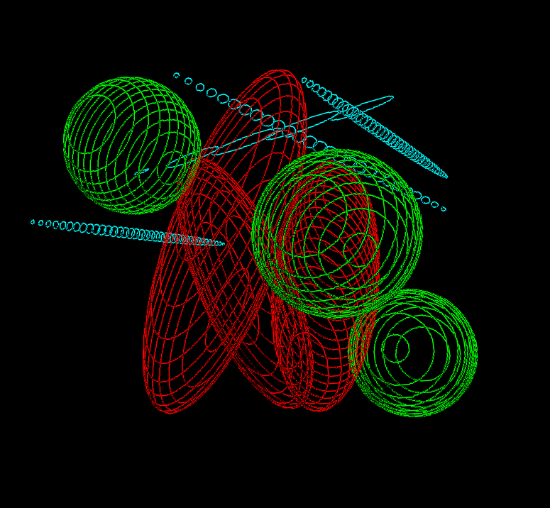
Currently, gensei (git version) supports generating images of more classes. For each class, the geometrical parameters, volume fraction, number of objects, and colour can be set separately. Moreover, the user can choose to generate series of sections in three perpendicular cutting planes. The following image contains objects of three classes (red, green, blue).

Objects of three classes.

Such a contrast image can be easily segmented. The following segmentation was performed with the Thresh module of the software Ellipse 3D (Vidito, KoĹĄice, Slovak Republic):

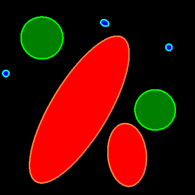
Segmentation.

The circumferences of all the object profiles can be saved and their geometrical properties (e.g., circularity, circumference, etc.) can be assessed. Moreover, the objects can be reconstructed in three dimensions after calibration and the contours can be visualized as follows (module Contours, software Ellipse 3D):

Contours.

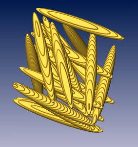
The surface of the objects can be reconstructed. The reconstruction gives usually best results when the objects were cut along their long axis. The following visualization was obtained with the Surface module of the software Ellipse 3D:

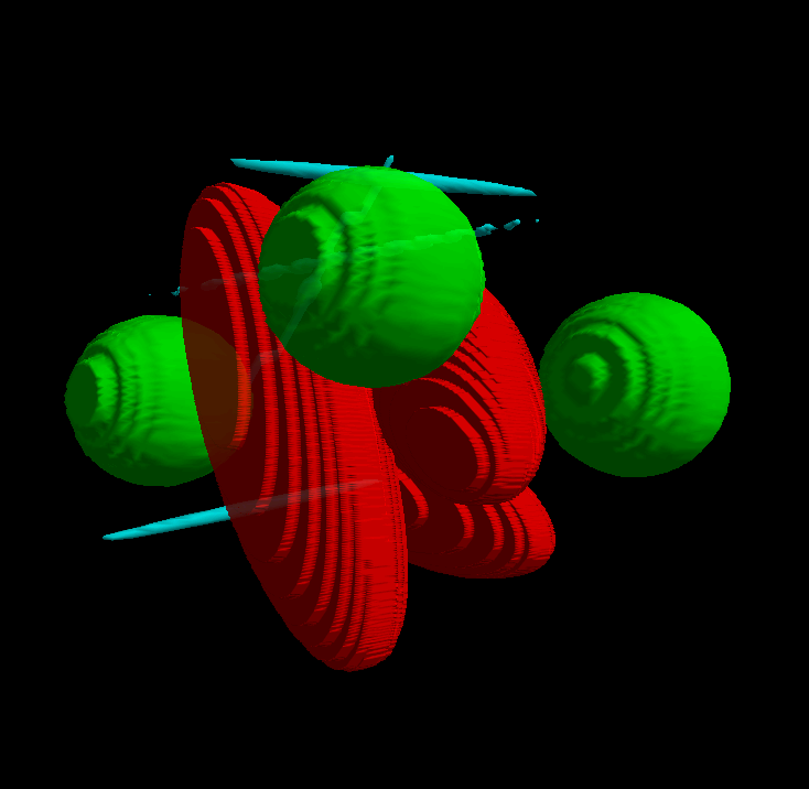
Surface.

The volume fraction and the surface of the objects is known and saved together with the image series. Therefore it can be used e.g. for training in histology - the trainee can compare the results of estimating the volume fraction (using the Cavalieri principle) either with the true volume fraction of the whole simulated objects or with the volume fraction based on the series of sections (the latter is usually lower as not all parts of the objects appear on the sections). Another application of the images is testing the settings of various stereological grids used for estimation of volume. When adjusting the geometrical parameters of stereological grids, it is usually desirable to find the lowest number of intersections between the objects and the grid, which still yields an acceptable amount of error. This minimum number of intersections depends on geometry of the objects, and the desired error (for details, see the nomogram published by Gundersen and Jensen, 1987). The user can easily check, whether the current settings give a good estimate of the true (known) volume. In the following example, the volume of red objects was quantified with a rectangular point grid (counted intersections are yellow, module LineSystem?, software Ellipse 3D):

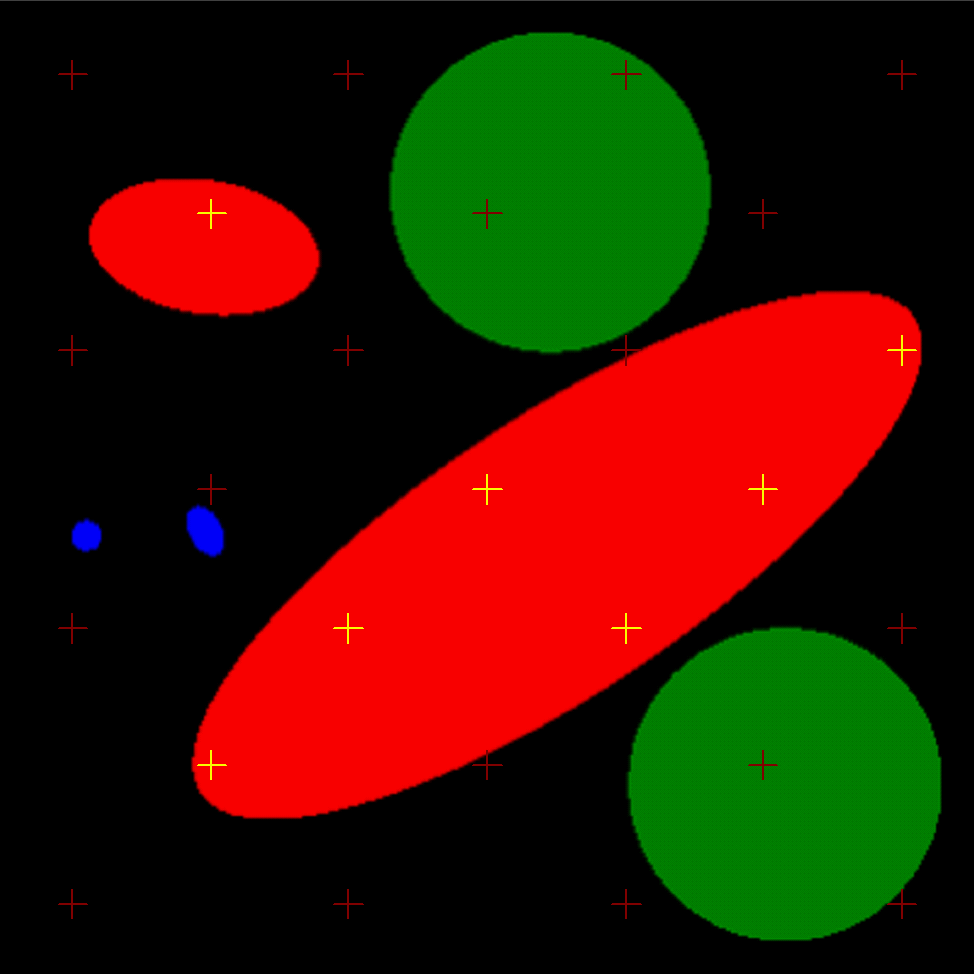
Red objects were quantified with a rectangular point grid.