Primer
A beginner’s tutorial highlighting the basics of SfePy.
Introduction
This primer presents a step-by-step walk-through of the process to solve a simple mechanics problem. The typical process to solve a problem using SfePy is followed: a model is meshed, a problem definition file is drafted, SfePy is run to solve the problem and finally the results of the analysis are visualised.
Problem statement
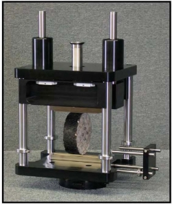
A popular test to measure the tensile strength of concrete or asphalt materials is the indirect tensile strength (ITS) test pictured below. In this test a cylindrical specimen is loaded across its diameter to failure. The test is usually run by loading the specimen at a constant deformation rate of 50 mm/minute (say) and measuring the load response. When the tensile stress that develops in the specimen under loading exceeds its tensile strength then the specimen will fail. To model this problem using finite elements the indirect tensile test can be simplified to represent a diametrically point loaded disk as shown in the schematic.
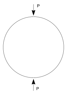
The tensile and compressive stresses that develop in the specimen as a
result of the point loads P are a function of the diameter  and
thickness
and
thickness  of the cylindrical specimen. At the centre of the
specimen, the compressive stress is 3 times the tensile stress and the
analytical formulation for these are, respectively:
of the cylindrical specimen. At the centre of the
specimen, the compressive stress is 3 times the tensile stress and the
analytical formulation for these are, respectively:
(1)
(2)
These solutions may be approximated using finite element methods. To solve this problem using SfePy the first step is meshing a suitable model.
Meshing
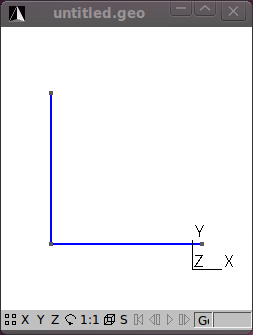
Assuming plane strain conditions, the indirect tensile test may be modelled using a 2D finite element mesh. Furthermore, the geometry of the model is symmetrical about the x- and y-axes passing through the centre of the circle. To take advantage of this symmetry only one quarter of the 2D model will be meshed and boundary conditions will be established to indicate this symmetry. The meshing program Gmsh is used here to very quickly mesh the model. Follow these steps to model the ITS, creating the file its2D.mesh <../meshes/2d/its2D.mesh>:
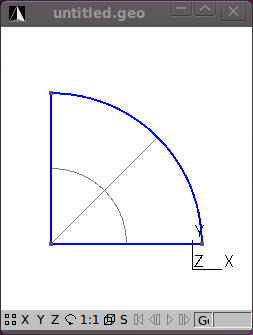
The ITS specimen has a diameter of 150 mm. Using Gmsh add (geometry/Elementary Entities/Add) three new points at the following coordinates:
 .
.Next add two straight lines connecting the points.
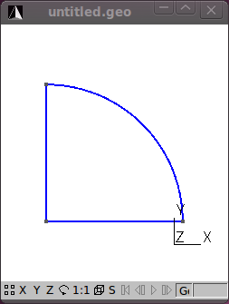
Next add a Circle arc connecting two of the points to form the quarter circle segment.
Still under Geometry/Elementary entities add a Plane Surface.
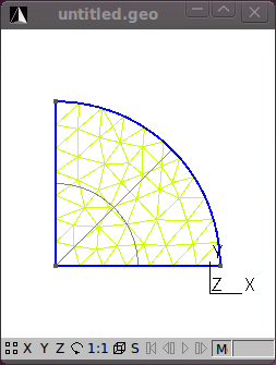
With the geometry of the model defined, add a mesh by clicking on the 2D button under the Mesh functions.
The figures that follow show the various stages in the model process.
That’s the meshing done. Save the mesh in a format that SfePy recognizes. For now use the medit .mesh format e.g. its2D.mesh.
Hint: Check the drop down in the Save As dialog for the different formats that Gmsh can save to.
If you open the its2D.mesh file using a text editor you’ll notice that
Gmsh saves the mesh in a 3D format and includes some extra geometry
items that should be deleted. Reformatted the mesh file to a 2D format
and delete the Edges block. Note that when you do this the file cannot
be reopened by Gmsh so it is always a good idea to also save your
meshes in Gmsh’s native format as well (Shift-Ctrl-S). Click
here to download the reformatted
mesh file that will be used in the tutorial.
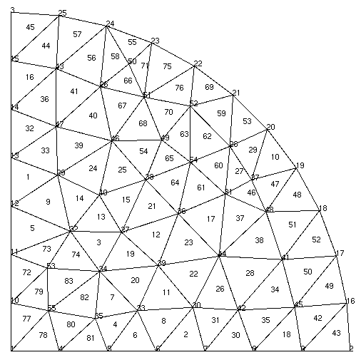
You’ll notice that the mesh contains 55 vertices (nodes) and 83 triangle elements. The mesh file provides the coordinates of the nodes and the element connectivity. It is important to note that node and element numbering in SfePy start at 0 and not 1 as is the case in Gmsh and some other meshing programs.
To view .mesh files you can use a demo of medit. After loading your mesh file with medit you can see the node and element numbering by pressing P and F respectively. The numbering in medit starts at 1 as shown. Thus the node at the center of the model in SfePy numbering is 0, and elements 76 and 77 are connected to this node. Node and element numbers can also be viewed in Gmsh – under the mesh option under the Visibility tab enable the node and surface labels. Note that the surface labels as numbered in Gmsh follow on from the line numbering. So to get the corresponding element number in SfePy you’ll need to subtract the number of lines in the Gmsh file + 1. Confused yet? Luckily, SfePy provides some useful mesh functions to indicate which elements are connected to which nodes. Nodes and elements can also be identified by defining regions, which is addressed later.
Another open source python option to view .mesh files is the appropriately named Python Mesh Viewer.
The next step in the process is coding the SfePy problem definition file.
Problem description
The programming of the problem description file is well documented in the SfePy User’s Guide. The problem description file used in the tutorial follows:
r"""
Diametrically point loaded 2-D disk. See :ref:`sec-primer`.

Find :math:`\ul{u}` such that:

.. math::
    \int_{\Omega} D_{ijkl}\ e_{ij}(\ul{v}) e_{kl}(\ul{u})
    = 0
    \;, \quad \forall \ul{v} \;,

where

.. math::
    D_{ijkl} = \mu (\delta_{ik} \delta_{jl}+\delta_{il} \delta_{jk}) +
    \lambda \ \delta_{ij} \delta_{kl}
    \;.
"""
from __future__ import absolute_import
from sfepy.mechanics.matcoefs import stiffness_from_youngpoisson
from sfepy.discrete.fem.utils import refine_mesh
from sfepy import data_dir

# Fix the mesh file name if you run this file outside the SfePy directory.
filename_mesh = data_dir + '/meshes/2d/its2D.mesh'

refinement_level = 0
filename_mesh = refine_mesh(filename_mesh, refinement_level)

output_dir = '.' # set this to a valid directory you have write access to

young = 2000.0 # Young's modulus [MPa]
poisson = 0.4  # Poisson's ratio

options = {
    'output_dir' : output_dir,
}

regions = {
    'Omega' : 'all',
    'Left' : ('vertices in (x < 0.001)', 'facet'),
    'Bottom' : ('vertices in (y < 0.001)', 'facet'),
    'Top' : ('vertex 2', 'vertex'),
}

materials = {
    'Asphalt' : ({'D': stiffness_from_youngpoisson(2, young, poisson)},),
    'Load' : ({'.val' : [0.0, -1000.0]},),
}

fields = {
    'displacement': ('real', 'vector', 'Omega', 1),
}

equations = {
   'balance_of_forces' :
   """dw_lin_elastic.2.Omega(Asphalt.D, v, u)
      = dw_point_load.0.Top(Load.val, v)""",
}

variables = {
    'u' : ('unknown field', 'displacement', 0),
    'v' : ('test field', 'displacement', 'u'),
}

ebcs = {
    'XSym' : ('Bottom', {'u.1' : 0.0}),
    'YSym' : ('Left', {'u.0' : 0.0}),
}

solvers = {
    'ls' : ('ls.scipy_direct', {}),
    'newton' : ('nls.newton', {
        'i_max' : 1,
        'eps_a' : 1e-6,
    }),
}
Download the Problem description file and open it in your favourite
Python editor. Note that you may wish to change the location of the output
directory to somewhere on your drive. You may also need to edit the mesh file
name. For the analysis we will assume that the material of the test specimen is
linear elastic and isotropic. We define two material constants i.e. Young’s
modulus and Poisson’s ratio. The material is assumed to be asphalt concrete
having a Young’s modulus of 2,000 MPa and a Poisson’s ration of 0.4.
Note: Be consistent in your choice and use of units. In the tutorial we are using Newton (N), millimeters (mm) and megaPascal (MPa). The sfepy.mechanics.units module might help you in determining which derived units correspond to given basic units.
The following block of code defines regions on your mesh:
regions = {
    'Omega' : 'all',
    'Left' : ('vertices in (x < 0.001)', 'facet'),
    'Bottom' : ('vertices in (y < 0.001)', 'facet'),
    'Top' : ('vertex 2', 'vertex'),
}
Four regions are defined:
‘Omega’: all the elements in the mesh,
‘Left’: the y-axis,
‘Bottom’: the x-axis,
‘Top’: the topmost node. This is where the load is applied.
Having defined the regions these can be used in other parts of your code. For example, in the definition of the boundary conditions:
ebcs = {
    'XSym' : ('Bottom', {'u.1' : 0.0}),
    'YSym' : ('Left', {'u.0' : 0.0}),
}
Now the power of the regions entity becomes apparent. To ensure symmetry about the x-axis, the vertical or y-displacement of the nodes in the ‘Bottom’ region are prevented or set to zero. Similarly, for symmetry about the y-axis, any horizontal or displacement in the x-direction of the nodes in the ‘Left’ region or y-axis is prevented.
The load is specified in terms of the ‘Load’ material as follows:
materials = {
    'Asphalt' : ({
        'lam' : lame_from_youngpoisson(young, poisson)[0],
        'mu' : lame_from_youngpoisson(young, poisson)[1],
    },),
    'Load' : ({'.val' : [0.0, -1000.0]},),
}
Note the dot in ‘.val’ – this denotes a special material value, i.e., a value that is not to be evaluated in quadrature points. The load is then applied in equations using the ‘dw_point_load.0.Top(Load.val, v)’ term in the topmost node (region ‘Top’).
We provided the material constants in terms of Young’s modulus and Poisson’s ratio, but the linear elastic isotropic equation used requires as input Lamé’s parameters. The lame_from_youngpoisson() function is thus used for conversion. Note that to use this function it was necessary to import the function into the code, which was done up front:
from sfepy.mechanics.matcoefs import lame_from_youngpoisson
Hint: Check out the sfepy.mechanics.matcoefs module for other useful material related functions.
That’s it – we are now ready to solve the problem.
Running SfePy
One option to solve the problem is to run the sfepy-run` command: from the command line:
sfepy-run its2D_1.py
Note: For the purpose of this tutorial it is assumed that the problem
description file (its2D_1.py) is in the current directory. If you have the
its2D_1.py file in another directory then make sure you include the path to
this file as well.
SfePy solves the problem and outputs the solution to the output path
(output_dir) provided in the script. The output file will be in the VTK
format by default if this is not explicitly specified and the name of
the output file will be the same as that used for the mesh file except
with the ‘.vtk’ extension i.e. its2D.vtk.
The VTK format is an ASCII format. Open the file using a text editor. You’ll notice that the output file includes separate sections:
POINTS (these are the model nodes),
CELLS (the model element connectivity),
VECTORS (the node displacements in the x-, y- and z- directions).
SfePy provides a script to quickly view the solution. To run this script you need to have pyvista installed. From the command line issue the following (assuming the correct paths):
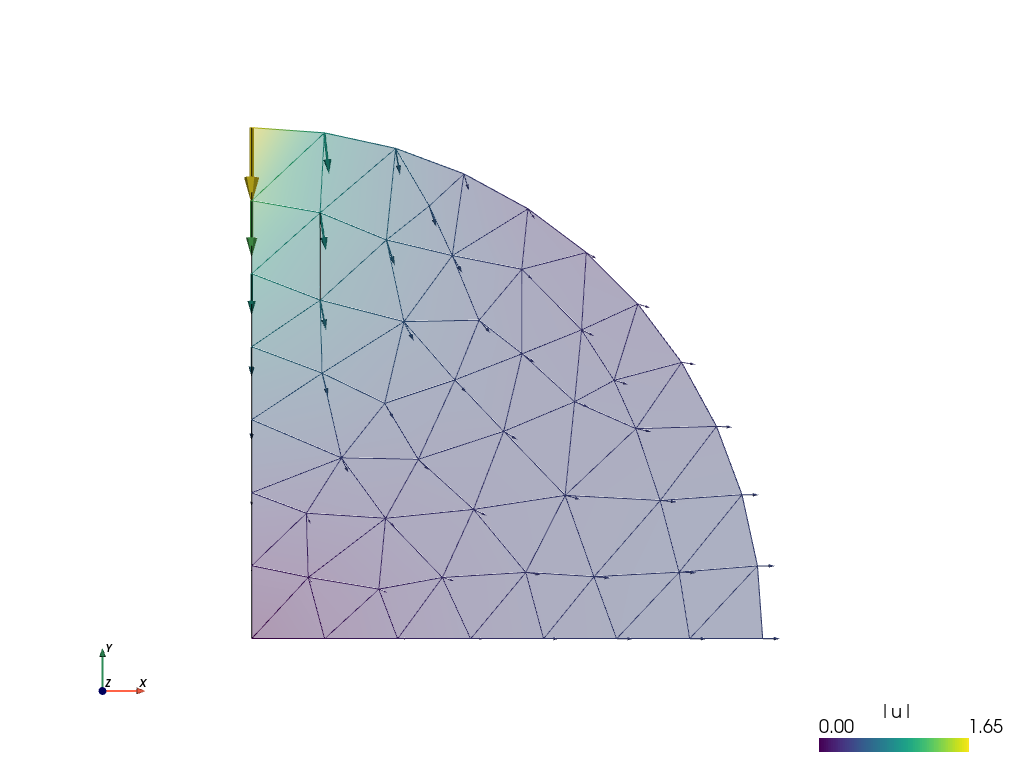
sfepy-view its2D.vtk -2 -e
The sfepy-view command generates the image shown below, which shows by default the displacements in the model as arrows and their magnitude as color scale. Cool, but we are more interested in the stresses. To get these we need to modify the problem description file and do some post-processing.
Post-processing
SfePy provides functions to calculate stresses and strains. We’ll
include a function to calculate these and update the problem material
definition and options to call this function as a
post_process_hook(). Save this file as its2D_2.py.
r"""
Diametrically point loaded 2-D disk with postprocessing. See
:ref:`sec-primer`.

Find :math:`\ul{u}` such that:

.. math::
    \int_{\Omega} D_{ijkl}\ e_{ij}(\ul{v}) e_{kl}(\ul{u})
    = 0
    \;, \quad \forall \ul{v} \;,

where

.. math::
    D_{ijkl} = \mu (\delta_{ik} \delta_{jl}+\delta_{il} \delta_{jk}) +
    \lambda \ \delta_{ij} \delta_{kl}
    \;.
"""

from __future__ import absolute_import
from sfepy.examples.linear_elasticity.its2D_1 import *

from sfepy.mechanics.matcoefs import stiffness_from_youngpoisson

def stress_strain(out, pb, state, extend=False):
    """
    Calculate and output strain and stress for given displacements.
    """
    from sfepy.base.base import Struct

    ev = pb.evaluate
    strain = ev('ev_cauchy_strain.2.Omega(u)', mode='el_avg')
    stress = ev('ev_cauchy_stress.2.Omega(Asphalt.D, u)', mode='el_avg',
                copy_materials=False)

    out['cauchy_strain'] = Struct(name='output_data', mode='cell',
                                  data=strain, dofs=None)
    out['cauchy_stress'] = Struct(name='output_data', mode='cell',
                                  data=stress, dofs=None)

    return out

asphalt = materials['Asphalt'][0]
asphalt.update({'D' : stiffness_from_youngpoisson(2, young, poisson)})
options.update({'post_process_hook' : 'stress_strain',})
The updated file imports all of the previous definitions in
its2D_1.py. The stress function (de_cauchy_stress()) requires as input
the stiffness tensor – thus it was necessary to update the materials
accordingly. The problem options were also updated to call the
stress_strain() function as a post_process_hook().
Run SfePy to solve the updated problem and view the solution (assuming the correct paths):
sfepy-run its2D_2.py
sfepy-view its2D.vtk -2 --max-plots 2
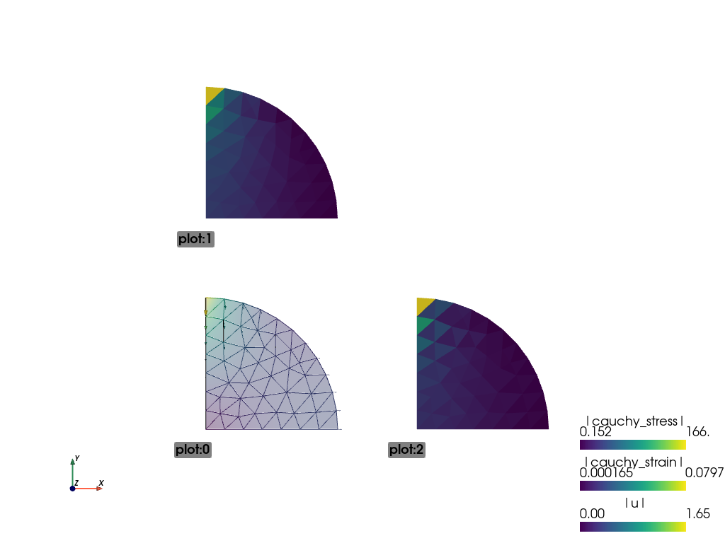
In addition to the node displacements, the VTK output shown below now also includes the stresses and strains averaged in the elements:
Remember the objective was to determine the stresses at the centre of
the specimen under a load  . The solution as currently derived is
expressed in terms of a global displacement vector
. The solution as currently derived is
expressed in terms of a global displacement vector  . The global
(residual) force vector
. The global
(residual) force vector  is a function of the global displacement
vector and the global stiffness matrix
is a function of the global displacement
vector and the global stiffness matrix  as:
as:  .
Let’s determine the force vector interactively.
.
Let’s determine the force vector interactively.
Running SfePy in interactive mode
In addition to solving problems using the sfepy-run command you can also run SfePy interactively (we will use IPython interactive shell in following examples).
In the SfePy top-level directory run
ipython
issue the following commands:
In [1]: from sfepy.applications import solve_pde

In [2]: pb, variables = solve_pde('its2D_2.py')
The problem is solved and the problem definition and solution are
provided in the pb and variables variables respectively. The solution,
or in this case, the global displacement vector , contains the x- and
y-displacements at the nodes in the 2D model:
In [3]: u = variables()

In [4]: u
Out[4]:
array([ 0.        ,  0.        ,  0.37376671, ..., -0.19923848,
        0.08820237, -0.11201528])

In [5]: u.shape
Out[5]: (110,)

In [6]: u.shape = (55, 2)

In [7]: u
Out[7]:
array([[ 0.        ,  0.        ],
       [ 0.37376671,  0.        ],
       [ 0.        , -1.65318152],
       ...,
       [ 0.08716448, -0.23069047],
       [ 0.27741356, -0.19923848],
       [ 0.08820237, -0.11201528]])
Note: We have used the fact, that the state vector contains only one variable (u). In general, the following can be used:
In [8]: u = variables.get_state_parts()['u']

In [9]: u
Out[9]:
array([[ 0.        ,  0.        ],
       [ 0.37376671,  0.        ],
       [ 0.        , -1.65318152],
       ...,
       [ 0.08716448, -0.23069047],
       [ 0.27741356, -0.19923848],
       [ 0.08820237, -0.11201528]])
Both variables() and variables.get_state_parts() return a view of the DOF
vector, that is why in Out[8] the vector is reshaped according to Out[6]. It is
thus possible to set the values of state variables by manipulating the state
vector, but shape changes such as the one above are not advised (see In
[15] below) - work on a copy instead.
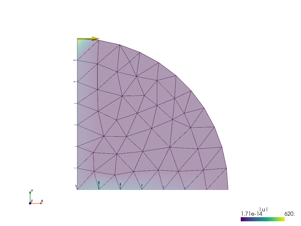
From the above it can be seen that u holds the displacements at the 55
nodes in the model and that the displacement at node 2 (on which the
load is applied) is 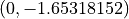 . The global stiffness
matrix is saved in pb as a sparse matrix:
. The global stiffness
matrix is saved in pb as a sparse matrix:
In [10]: K = pb.mtx_a
In [11]: K
Out[11]:
<94x94 sparse matrix of type '<type 'numpy.float64'>'
with 1070 stored elements in Compressed Sparse Row format>
In [12]: print(K)
(0, 0) 2443.95959851
(0, 7) -2110.99917491
(0, 14) -332.960423597
(0, 15) 1428.57142857
(1, 1) 2443.95959852
(1, 13) -2110.99917492
(1, 32) 1428.57142857
(1, 33) -332.960423596
(2, 2) 4048.78343529
(2, 3) -1354.87004384
(2, 52) -609.367453538
(2, 53) -1869.0018791
(2, 92) -357.41672785
(2, 93) 1510.24654193
(3, 2) -1354.87004384
(3, 3) 4121.03202907
(3, 4) -1696.54911732
(3, 48) 76.2400806561
(3, 49) -1669.59247304
(3, 52) -1145.85294856
(3, 53) 2062.13955556
(4, 3) -1696.54911732
(4, 4) 4410.17902905
(4, 5) -1872.87344838
(4, 42) -130.515009576
: :
(91, 81) -1610.0550578
(91, 86) -199.343680224
(91, 87) -2330.41406097
(91, 90) -575.80373408
(91, 91) 7853.23899229
(92, 2) -357.41672785
(92, 8) 1735.59411191
(92, 50) -464.976034459
(92, 51) -1761.31189004
(92, 52) -3300.45367361
(92, 53) 1574.59387937
(92, 88) -250.325600254
(92, 89) 1334.11823335
(92, 92) 9219.18643706
(92, 93) -2607.52659081
(93, 2) 1510.24654193
(93, 8) -657.361661955
(93, 50) -1761.31189004
(93, 51) 54.1134516246
(93, 52) 1574.59387937
(93, 53) -315.793227627
(93, 88) 1334.11823335
(93, 89) -4348.13351285
(93, 92) -2607.52659081
(93, 93) 9821.16012014
In [13]: K.shape
Out[13]: (94, 94)
One would expect the shape of the global stiffness matrix to be
 i.e. to have the same number of rows and columns as u. This
matrix has been reduced by the fixed degrees of freedom imposed by the
boundary conditions set at the nodes on symmetry axes. To restore the
shape of the matrix, temporarily remove the imposed boundary conditions:
i.e. to have the same number of rows and columns as u. This
matrix has been reduced by the fixed degrees of freedom imposed by the
boundary conditions set at the nodes on symmetry axes. To restore the
shape of the matrix, temporarily remove the imposed boundary conditions:
In [14]: pb.remove_bcs()
Note that the matrix is reallocated, so it contains only zeros at this moment.
Now we can calculate the force vector :
In [15]: f = pb.evaluator.eval_residual(u)
This leads to:
ValueError: shape mismatch: value array of shape (55,2) could not be broadcast to indexing result of shape (110,)
– the original shape of the DOF vector needs to be restored:
In [16]: u.shape = variables.vec.shape = (110,)

In [17]: f = pb.evaluator.eval_residual(u)


In [18]: f.shape
Out[18]: (110,)

In [19]: f
Out[19]:
array([ -4.73618436e+01,   1.42752386e+02,   1.56921124e-13, ...,
        -2.06057393e-13,   2.13162821e-14,  -2.84217094e-14])
Remember to restore the original boundary conditions previously removed in step [14]:
In [20]: pb.time_update()
To view the residual force vector, we can save it to a VTK file. This requires setting f to (a copy of) the variables as follows:
In [21]: fvars = variables.copy() # Shallow copy, .vec is shared!
In [22]: fvars.init_state(f) # Initialize new .vec with f.
In [23]: out = fvars.create_output()
In [24]: pb.save_state('file.vtk', out=out)
Running the sfepy-view command on file.vtk, i.e.
In [25]: ! sfepy-view file.vtk
displays the average nodal forces as shown below:
The forces in the x- and y-directions at node 2 are:
In [26]: f.shape = (55, 2)
In [27]: f[2]
Out[27]: array([  6.20373272e+02,  -1.13686838e-13])
Great, we have an almost zero residual vertical load or force apparent at node 2 i.e. -1.13686838e-13 Newton. Note that these relatively very small numbers can be slightly different, depending on the linear solver kind and version.
Let us now check the stress at node 0, the centre of the specimen.
Generating output at element nodes
Previously we had calculated the stresses in the model but these were
averaged from those calculated at Gauss quadrature points within the
elements. It is possible to provide custom integrals to allow the
calculation of stresses with the Gauss quadrature points at the element
nodes. This will provide us a more accurate estimate of the stress at
the centre of the specimen located at node 0. The code below outlines one way to
achieve this.
r"""
Diametrically point loaded 2-D disk with nodal stress calculation. See
:ref:`sec-primer`.

Find :math:`\ul{u}` such that:

.. math::
    \int_{\Omega} D_{ijkl}\ e_{ij}(\ul{v}) e_{kl}(\ul{u})
    = 0
    \;, \quad \forall \ul{v} \;,

where

.. math::
    D_{ijkl} = \mu (\delta_{ik} \delta_{jl}+\delta_{il} \delta_{jk}) +
    \lambda \ \delta_{ij} \delta_{kl}
    \;.
"""
from __future__ import print_function
from __future__ import absolute_import
from sfepy.examples.linear_elasticity.its2D_1 import *

from sfepy.mechanics.matcoefs import stiffness_from_youngpoisson
from sfepy.discrete.fem.geometry_element import geometry_data
from sfepy.discrete import FieldVariable
from sfepy.discrete.fem import Field
import numpy as nm

gdata = geometry_data['2_3']
nc = len(gdata.coors)

def nodal_stress(out, pb, state, extend=False, integrals=None):
    '''
    Calculate stresses at nodal points.
    '''

    # Point load.
    mat = pb.get_materials()['Load']
    P = 2.0 * mat.get_data('special', 'val')[1]

    # Calculate nodal stress.
    pb.time_update()

    if integrals is None: integrals = pb.get_integrals()

    stress = pb.evaluate('ev_cauchy_stress.ivn.Omega(Asphalt.D, u)', mode='qp',
                         integrals=integrals, copy_materials=False)
    sfield = Field.from_args('stress', nm.float64, (3,),
                             pb.domain.regions['Omega'])
    svar = FieldVariable('sigma', 'parameter', sfield,
                         primary_var_name='(set-to-None)')
    svar.set_from_qp(stress, integrals['ivn'])

    print('\n==================================================================')
    print('Given load = %.2f N' % -P)
    print('\nAnalytical solution')
    print('===================')
    print('Horizontal tensile stress = %.5e MPa/mm' % (-2.*P/(nm.pi*150.)))
    print('Vertical compressive stress = %.5e MPa/mm' % (-6.*P/(nm.pi*150.)))
    print('\nFEM solution')
    print('============')
    print('Horizontal tensile stress = %.5e MPa/mm' % (svar()[0]))
    print('Vertical compressive stress = %.5e MPa/mm' % (-svar()[1]))
    print('==================================================================')
    return out

asphalt = materials['Asphalt'][0]
asphalt.update({'D' : stiffness_from_youngpoisson(2, young, poisson)})
options.update({'post_process_hook' : 'nodal_stress',})

integrals = {
    'ivn' : ('custom', gdata.coors, [gdata.volume / nc] * nc),
}
The output:
==================================================================
Given load = 2000.00 N

Analytical solution
===================
Horizontal tensile stress = 8.48826e+00 MPa/mm
Vertical compressive stress = 2.54648e+01 MPa/mm

FEM solution
============
Horizontal tensile stress = 7.57220e+00 MPa/mm
Vertical compressive stress = 2.58660e+01 MPa/mm
==================================================================
Not bad for such a coarse mesh! Re-running the problem using a
finer mesh provides a more accurate
solution:
==================================================================
Given load = 2000.00 N

Analytical solution
===================
Horizontal tensile stress = 8.48826e+00 MPa/mm
Vertical compressive stress = 2.54648e+01 MPa/mm

FEM solution
============
Horizontal tensile stress = 8.50042e+00 MPa/mm
Vertical compressive stress = 2.54300e+01 MPa/mm
To see how the FEM solution approaches the analytical one, try to play with the uniform mesh refinement level in the Problem description file, namely lines 25, 26:
refinement_level = 0
filename_mesh = refine_mesh(filename_mesh, refinement_level)
The above computation could also be done in the IPython shell:
In [23]: from sfepy.applications import solve_pde
In [24]: from sfepy.discrete import (Field, FieldVariable, Material,
                                     Integral, Integrals)
In [25]: from sfepy.discrete.fem.geometry_element import geometry_data

In [26]: gdata = geometry_data['2_3']
In [27]: nc = len(gdata.coors)
In [28]: ivn = Integral('ivn', order=-1,
   ....:                coors=gdata.coors, weights=[gdata.volume / nc] * nc)

In [29]: pb, variables = solve_pde('sfepy/examples/linear_elasticity/its2D_2.py')

In [30]: stress = pb.evaluate('ev_cauchy_stress.ivn.Omega(Asphalt.D,u)',
   ....:                      mode='qp', integrals=Integrals([ivn]))
In [31]: sfield = Field.from_args('stress', nm.float64, (3,), pb.domain.regions['Omega'])
In [32]: svar = FieldVariable('sigma', 'parameter', sfield,
   ....:                      primary_var_name='(set-to-None)')
In [33]: svar.set_from_qp(stress, ivn)

In [34]: print('Horizontal tensile stress = %.5e MPa/mm' % (svar()[0]))
Horizontal tensile stress = 7.57220e+00 MPa/mm
In [35]: print('Vertical compressive stress = %.5e MPa/mm' % (-svar()[1]))
Vertical compressive stress = 2.58660e+01 MPa/mm

In [36]: mat = pb.get_materials()['Load']
In [37]: P = 2.0 * mat.get_data('special', 'val')[1]
In [38]: P
Out[38]: -2000.0

In [39]: print('Horizontal tensile stress = %.5e MPa/mm' % (-2.*P/(nm.pi*150.)))
Horizontal tensile stress = 8.48826e+00 MPa/mm
In [40]: print('Vertical compressive stress = %.5e MPa/mm' % (-6.*P/(nm.pi*150.)))
Vertical compressive stress = 2.54648e+01 MPa/mm
To wrap this tutorial up let’s explore SfePy’s probing functions.
Probing
As a bonus for sticking to the end of this tutorial see the following
Problem description file that provides SfePy
functions to quickly and neatly probe the solution.
r"""
Diametrically point loaded 2-D disk with postprocessing and probes. See
:ref:`sec-primer`.

Find :math:`\ul{u}` such that:

.. math::
    \int_{\Omega} D_{ijkl}\ e_{ij}(\ul{v}) e_{kl}(\ul{u})
    = 0
    \;, \quad \forall \ul{v} \;,

where

.. math::
    D_{ijkl} = \mu (\delta_{ik} \delta_{jl}+\delta_{il} \delta_{jk}) +
    \lambda \ \delta_{ij} \delta_{kl}
    \;.
"""
from __future__ import absolute_import
from sfepy.examples.linear_elasticity.its2D_1 import *

from sfepy.mechanics.matcoefs import stiffness_from_youngpoisson
from sfepy.postprocess.probes_vtk import Probe

import os
from six.moves import range

def stress_strain(out, pb, state, extend=False):
    """
    Calculate and output strain and stress for given displacements.
    """
    from sfepy.base.base import Struct
    import matplotlib.pyplot as plt
    import matplotlib.font_manager as fm

    ev = pb.evaluate
    strain = ev('ev_cauchy_strain.2.Omega(u)', mode='el_avg')
    stress = ev('ev_cauchy_stress.2.Omega(Asphalt.D, u)', mode='el_avg')

    out['cauchy_strain'] = Struct(name='output_data', mode='cell',
                                  data=strain, dofs=None)
    out['cauchy_stress'] = Struct(name='output_data', mode='cell',
                                  data=stress, dofs=None)

    probe = Probe(out, pb.domain.mesh, probe_view=True)

    ps0 = [[0.0,  0.0, 0.0], [ 0.0,  0.0, 0.0]]
    ps1 = [[75.0, 0.0, 0.0], [ 0.0, 75.0, 0.0]]
    n_point = 10

    labels = ['%s -> %s' % (p0, p1) for p0, p1 in zip(ps0, ps1)]
    probes = []
    for ip in range(len(ps0)):
        p0, p1 = ps0[ip], ps1[ip]
        probes.append('line%d' % ip)
        probe.add_line_probe('line%d' % ip, p0, p1, n_point)

    for ip, label in zip(probes, labels):
        fig = plt.figure()
        plt.clf()
        fig.subplots_adjust(hspace=0.4)
        plt.subplot(311)
        pars, vals = probe(ip, 'u')
        for ic in range(vals.shape[1] - 1):
            plt.plot(pars, vals[:,ic], label=r'$u_{%d}$' % (ic + 1),
                     lw=1, ls='-', marker='+', ms=3)
        plt.ylabel('displacements')
        plt.xlabel('probe %s' % label, fontsize=8)
        plt.legend(loc='best', prop=fm.FontProperties(size=10))

        sym_labels = ['11', '22', '12']

        plt.subplot(312)
        pars, vals = probe(ip, 'cauchy_strain')
        for ii in range(vals.shape[1]):
            plt.plot(pars, vals[:, ii], label=r'$e_{%s}$' % sym_labels[ii],
                     lw=1, ls='-', marker='+', ms=3)
        plt.ylabel('Cauchy strain')
        plt.xlabel('probe %s' % label, fontsize=8)
        plt.legend(loc='best', prop=fm.FontProperties(size=8))

        plt.subplot(313)
        pars, vals = probe(ip, 'cauchy_stress')
        for ii in range(vals.shape[1]):
            plt.plot(pars, vals[:, ii], label=r'$\sigma_{%s}$' % sym_labels[ii],
                     lw=1, ls='-', marker='+', ms=3)
        plt.ylabel('Cauchy stress')
        plt.xlabel('probe %s' % label, fontsize=8)
        plt.legend(loc='best', prop=fm.FontProperties(size=8))

        opts = pb.conf.options
        filename_results = os.path.join(opts.get('output_dir'),
                                        'its2D_probe_%s.png' % ip)

        fig.savefig(filename_results)

    return out

materials['Asphalt'][0].update({'D' : stiffness_from_youngpoisson(2, young, poisson)})

options.update({
    'post_process_hook' : 'stress_strain',
})
Probing applies interpolation to output the solution along specified paths. For the tutorial, line probing is done along the x- and y-axes of the model.
Run SfePy to solve the problem and apply the probes:
sfepy-run its2D_5.py
The probing function will generate the following figures that show the displacements, normal stresses and strains as well as shear stresses and strains along the probe paths. Note that you need matplotlib installed to run this example.
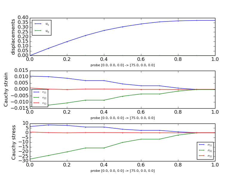
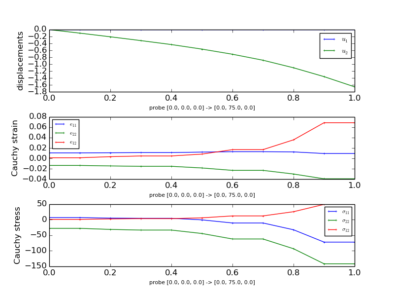
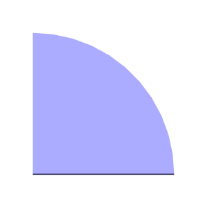
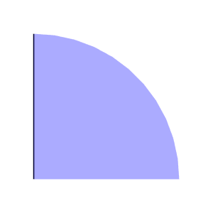
The probing function also generates previews of the mesh with the probe paths.
Interactive Example
SfePy can be used also interactively by constructing directly the classes that corresponds to the keywords in the problem description files. The following listing shows a script with the same (and more) functionality as the above examples:
#!/usr/bin/env python
"""
Diametrically point loaded 2-D disk, using commands for interactive use. See
:ref:`sec-primer`.

The script combines the functionality of all the ``its2D_?.py`` examples and
allows setting various simulation parameters, namely:

- material parameters
- displacement field approximation order
- uniform mesh refinement level

The example shows also how to probe the results as in
:ref:`linear_elasticity-its2D_4`. Using :mod:`sfepy.discrete.probes` allows
correct probing of fields with the approximation order greater than one.

In the SfePy top-level directory the following command can be used to get usage
information::

  python sfepy/examples/linear_elasticity/its2D_interactive.py -h
"""
from __future__ import absolute_import
import sys
from six.moves import range
sys.path.append('.')
from argparse import ArgumentParser, RawDescriptionHelpFormatter

import numpy as nm
import matplotlib.pyplot as plt

from sfepy.base.base import assert_, output, ordered_iteritems, IndexedStruct
from sfepy.discrete import (FieldVariable, Material, Integral, Integrals,
                            Equation, Equations, Problem)
from sfepy.discrete.fem import Mesh, FEDomain, Field
from sfepy.terms import Term
from sfepy.discrete.conditions import Conditions, EssentialBC
from sfepy.mechanics.matcoefs import stiffness_from_youngpoisson
from sfepy.solvers.auto_fallback import AutoDirect
from sfepy.solvers.nls import Newton
from sfepy.discrete.fem.geometry_element import geometry_data
from sfepy.discrete.probes import LineProbe
from sfepy.discrete.projections import project_by_component

from sfepy.examples.linear_elasticity.its2D_2 import stress_strain
from sfepy.examples.linear_elasticity.its2D_3 import nodal_stress

def gen_lines(problem):
    """
    Define two line probes.

    Additional probes can be added by appending to `ps0` (start points) and
    `ps1` (end points) lists.
    """
    ps0 = [[0.0,  0.0], [0.0,  0.0]]
    ps1 = [[75.0, 0.0], [0.0, 75.0]]

    # Use enough points for higher order approximations.
    n_point = 1000

    labels = ['%s -> %s' % (p0, p1) for p0, p1 in zip(ps0, ps1)]
    probes = []
    for ip in range(len(ps0)):
        p0, p1 = ps0[ip], ps1[ip]
        probes.append(LineProbe(p0, p1, n_point))

    return probes, labels

def probe_results(u, strain, stress, probe, label):
    """
    Probe the results using the given probe and plot the probed values.
    """
    results = {}

    pars, vals = probe(u)
    results['u'] = (pars, vals)
    pars, vals = probe(strain)
    results['cauchy_strain'] = (pars, vals)
    pars, vals = probe(stress)
    results['cauchy_stress'] = (pars, vals)

    fig = plt.figure()
    plt.clf()
    fig.subplots_adjust(hspace=0.4)
    plt.subplot(311)
    pars, vals = results['u']
    for ic in range(vals.shape[1]):
        plt.plot(pars, vals[:,ic], label=r'$u_{%d}$' % (ic + 1),
                 lw=1, ls='-', marker='+', ms=3)
    plt.ylabel('displacements')
    plt.xlabel('probe %s' % label, fontsize=8)
    plt.legend(loc='best', fontsize=10)

    sym_indices = ['11', '22', '12']

    plt.subplot(312)
    pars, vals = results['cauchy_strain']
    for ic in range(vals.shape[1]):
        plt.plot(pars, vals[:,ic], label=r'$e_{%s}$' % sym_indices[ic],
                 lw=1, ls='-', marker='+', ms=3)
    plt.ylabel('Cauchy strain')
    plt.xlabel('probe %s' % label, fontsize=8)
    plt.legend(loc='best', fontsize=10)

    plt.subplot(313)
    pars, vals = results['cauchy_stress']
    for ic in range(vals.shape[1]):
        plt.plot(pars, vals[:,ic], label=r'$\sigma_{%s}$' % sym_indices[ic],
                 lw=1, ls='-', marker='+', ms=3)
    plt.ylabel('Cauchy stress')
    plt.xlabel('probe %s' % label, fontsize=8)
    plt.legend(loc='best', fontsize=10)

    return fig, results

helps = {
    'young' : "the Young's modulus [default: %(default)s]",
    'poisson' : "the Poisson's ratio [default: %(default)s]",
    'load' : "the vertical load value (negative means compression)"
    " [default: %(default)s]",
    'order' : 'displacement field approximation order [default: %(default)s]',
    'refine' : 'uniform mesh refinement level [default: %(default)s]',
    'probe' : 'probe the results',
}

def main():
    from sfepy import data_dir

    parser = ArgumentParser(description=__doc__,
                            formatter_class=RawDescriptionHelpFormatter)
    parser.add_argument('--version', action='version', version='%(prog)s')
    parser.add_argument('--young', metavar='float', type=float,
                      action='store', dest='young',
                      default=2000.0, help=helps['young'])
    parser.add_argument('--poisson', metavar='float', type=float,
                      action='store', dest='poisson',
                      default=0.4, help=helps['poisson'])
    parser.add_argument('--load', metavar='float', type=float,
                      action='store', dest='load',
                      default=-1000.0, help=helps['load'])
    parser.add_argument('--order', metavar='int', type=int,
                      action='store', dest='order',
                      default=1, help=helps['order'])
    parser.add_argument('-r', '--refine', metavar='int', type=int,
                      action='store', dest='refine',
                      default=0, help=helps['refine'])
    parser.add_argument('-p', '--probe',
                      action="store_true", dest='probe',
                      default=False, help=helps['probe'])
    options = parser.parse_args()

    assert_((0.0 < options.poisson < 0.5),
            "Poisson's ratio must be in ]0, 0.5[!")
    assert_((0 < options.order),
            'displacement approximation order must be at least 1!')

    output('using values:')
    output("  Young's modulus:", options.young)
    output("  Poisson's ratio:", options.poisson)
    output('  vertical load:', options.load)
    output('uniform mesh refinement level:', options.refine)

    # Build the problem definition.
    mesh = Mesh.from_file(data_dir + '/meshes/2d/its2D.mesh')
    domain = FEDomain('domain', mesh)

    if options.refine > 0:
        for ii in range(options.refine):
            output('refine %d...' % ii)
            domain = domain.refine()
            output('... %d nodes %d elements'
                   % (domain.shape.n_nod, domain.shape.n_el))

    omega = domain.create_region('Omega', 'all')
    left = domain.create_region('Left',
                                'vertices in x < 0.001', 'facet')
    bottom = domain.create_region('Bottom',
                                  'vertices in y < 0.001', 'facet')
    top = domain.create_region('Top', 'vertex 2', 'vertex')

    field = Field.from_args('fu', nm.float64, 'vector', omega,
                            approx_order=options.order)

    u = FieldVariable('u', 'unknown', field)
    v = FieldVariable('v', 'test', field, primary_var_name='u')

    D = stiffness_from_youngpoisson(2, options.young, options.poisson)

    asphalt = Material('Asphalt', D=D)
    load = Material('Load', values={'.val' : [0.0, options.load]})

    integral = Integral('i', order=2*options.order)
    integral0 = Integral('i', order=0)

    t1 = Term.new('dw_lin_elastic(Asphalt.D, v, u)',
                  integral, omega, Asphalt=asphalt, v=v, u=u)
    t2 = Term.new('dw_point_load(Load.val, v)',
                  integral0, top, Load=load, v=v)
    eq = Equation('balance', t1 - t2)
    eqs = Equations([eq])

    xsym = EssentialBC('XSym', bottom, {'u.1' : 0.0})
    ysym = EssentialBC('YSym', left, {'u.0' : 0.0})

    ls = AutoDirect({})

    nls_status = IndexedStruct()
    nls = Newton({}, lin_solver=ls, status=nls_status)

    pb = Problem('elasticity', equations=eqs)

    pb.set_bcs(ebcs=Conditions([xsym, ysym]))

    pb.set_solver(nls)

    # Solve the problem.
    variables = pb.solve()
    output(nls_status)

    # Postprocess the solution.
    out = variables.create_output()
    out = stress_strain(out, pb, variables, extend=True)
    pb.save_state('its2D_interactive.vtk', out=out)

    gdata = geometry_data['2_3']
    nc = len(gdata.coors)

    integral_vn = Integral('ivn', coors=gdata.coors,
                          weights=[gdata.volume / nc] * nc)

    nodal_stress(out, pb, variables, integrals=Integrals([integral_vn]))

    if options.probe:
        # Probe the solution.
        probes, labels = gen_lines(pb)

        sfield = Field.from_args('sym_tensor', nm.float64, 3, omega,
                                approx_order=options.order - 1)
        stress = FieldVariable('stress', 'parameter', sfield,
                               primary_var_name='(set-to-None)')
        strain = FieldVariable('strain', 'parameter', sfield,
                               primary_var_name='(set-to-None)')

        cfield = Field.from_args('component', nm.float64, 1, omega,
                                 approx_order=options.order - 1)
        component = FieldVariable('component', 'parameter', cfield,
                                  primary_var_name='(set-to-None)')

        ev = pb.evaluate
        order = 2 * (options.order - 1)
        strain_qp = ev('ev_cauchy_strain.%d.Omega(u)' % order, mode='qp')
        stress_qp = ev('ev_cauchy_stress.%d.Omega(Asphalt.D, u)' % order,
                       mode='qp', copy_materials=False)

        project_by_component(strain, strain_qp, component, order)
        project_by_component(stress, stress_qp, component, order)

        all_results = []
        for ii, probe in enumerate(probes):
            fig, results = probe_results(u, strain, stress, probe, labels[ii])

            fig.savefig('its2D_interactive_probe_%d.png' % ii)
            all_results.append(results)

        for ii, results in enumerate(all_results):
            output('probe %d:' % ii)
            output.level += 2
            for key, res in ordered_iteritems(results):
                output(key + ':')
                val = res[1]
                output('  min: %+.2e, mean: %+.2e, max: %+.2e'
                       % (val.min(), val.mean(), val.max()))
            output.level -= 2


if __name__ == '__main__':
    main()
The script can be run from the SfePy top-level directory, assuming the in-place build, as follows:
python sfepy/examples/linear_elasticity/its2D_interactive.py
The script allows setting several parameters that influence the solution, see:
python sfepy/examples/linear_elasticity/its2D_interactive.py -h
for the complete list. Besides the material parameters, a uniform mesh refinement level and the displacement field approximation order can be specified. The script demonstrates how to
project a derived quantity, that is evaluated in quadrature points (e.g. a strain or stress), into a field variable;
probe the solution defined in the field variables.
Using sfepy.discrete.probes allows correct probing of fields with the
approximation order greater than one.
The end.