Material Identification
Introduction
This tutorial shows identification of material parameters of a composite structure using data (force-displacement curves) obtained by a standard tensile test.
Composite structure
The unidirectional long fiber carbon-epoxy composite is considered. Its microstructure was analysed by the scanning electron microscopy and the data, volume fractions and fibers cross-sections, were used to generate a periodic finite element mesh (representative volume element - RVE) representing the random composite structure at the microscopic level (the random structure generation algorithm is described in [1]):
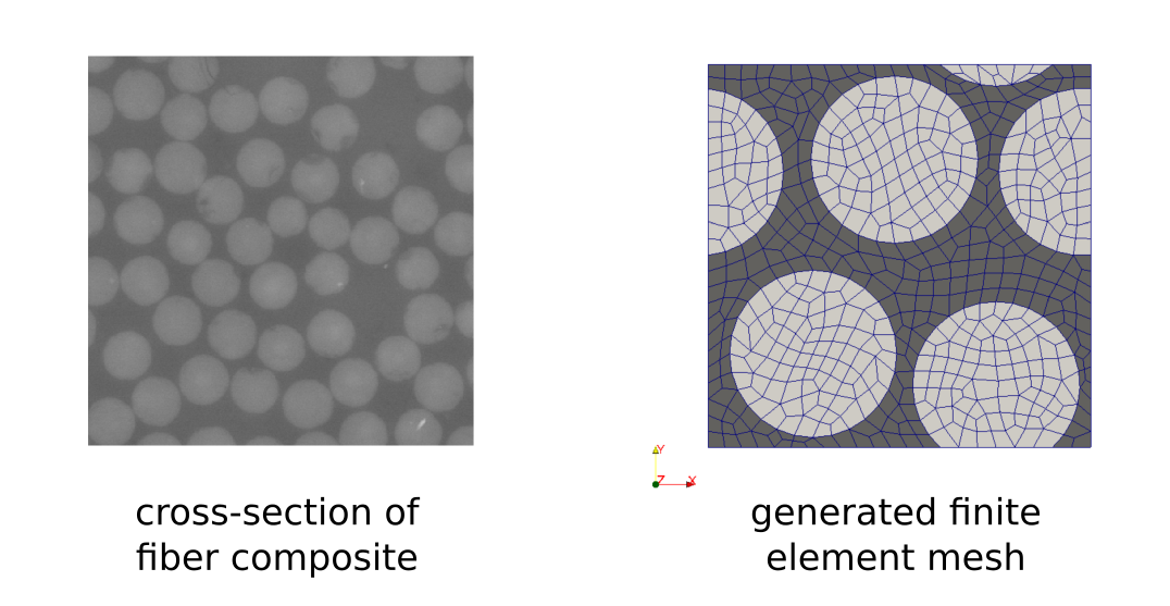
This RVE is used in the micromechanical FE analysis which is based on the two-scale homogenization method.
Material testing
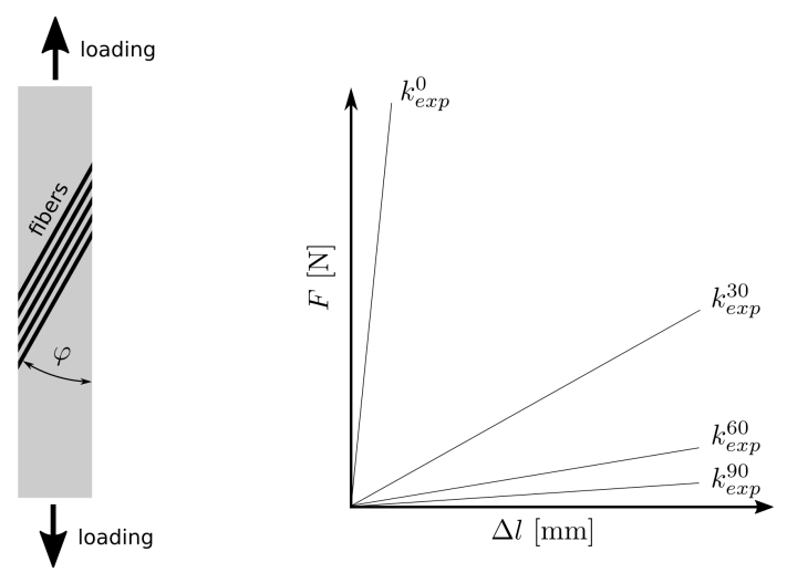
Several carbon-expoxy specimens with different fiber orientations (0, 30, 60 and 90 degrees) were subjected to the tensile test in order to obtain force-elongation dependencies, see [2]. The slopes of the linearized dependencies were used in an objective function of the identification process.
Numerical simulation
The linear isotropic material model is used for both components (fiber and matrix) of the composite so only four material parameters (Young’s modulus and Poisson’s ratio for each component) are necessary to fully describe the mechanical behavior of the structure.
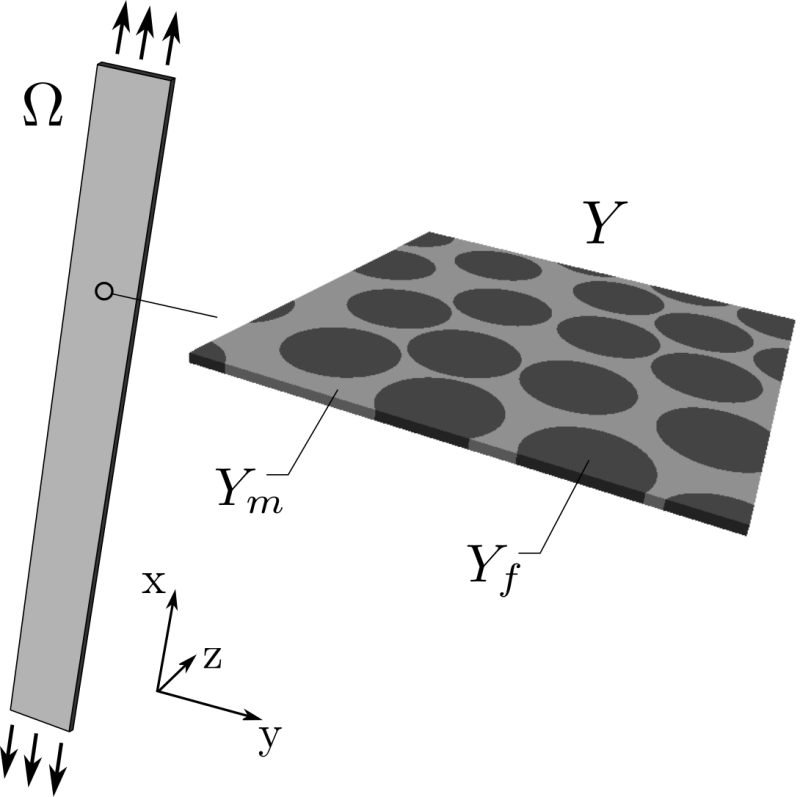
The numerical simulations of the tensile tests are based on the homogenization method applied to the linear elastic problem [3]. The homogenization procedure results in the microscopic problem solved within the RVE and the macroscopic problem that involves the homogenized elastic coefficients.
Homogenized coefficients
The problem at the microscopic level is formulated in terms of characteristic response functions and its solution is used to evaluate the homogenized elasticity tensor. The microscopic problem has to be solved with the periodic boundary conditions.
The following SfePy description file is used for definition of the microscopic problem: homogenization_opt.py.
In the case of the identification process function get_mat() obtains the material parameters (Young’s modules, Poisson’s ratios) from the outer identification loop. Otherwise these parameters are given by values.
Notice the use of parametric_hook (Miscellaneous) to pass
around the optimization parameters.
Macroscopic simulation
The homogenized elasticity problem is solved for the unknown macroscopic displacements and the elongation of the composite specimen is evaluated for a given loading. These values are used to determine the slopes of the calculated force-elongation dependencies which are required by the objective function.
The SfePy description file for the macroscopic analysis: linear_elasticity_opt.py.
Identification procedure
The identification of material parameters, i.e. the Young’s modulus and
Poisson’s ratio, of the epoxy matrix ( ,
,  ) and carbon
fibers (
) and carbon
fibers ( ,
,  ) can be formulated as a minimization of the
following objective function:
) can be formulated as a minimization of the
following objective function:
(1)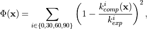
where  and
and  are the computed and measured
slopes of the force-elongation tangent lines for a given fiber orientation. This
function is minimized using scipy.optimize.fmin_tnc(), considering bounds of
the identified parameters.
are the computed and measured
slopes of the force-elongation tangent lines for a given fiber orientation. This
function is minimized using scipy.optimize.fmin_tnc(), considering bounds of
the identified parameters.
Tho following steps are performed in each iteration of the optimization loop:
Solution of the microscopic problem, evaluation of the homogenized elasticity tensor.
Solution of the macroscopic problems for different fiber orientations (0, 30, 60, 90), this is incorporated by appropriate rotation of the elasticity tensor.
Evaluation of the objective function.
Python script for material identification: material_opt.py.
Running identification script
Run the script from the command shell as (from the top-level directory of SfePy):
$ python sfepy/examples/homogenization/material_opt.py
The iteration process is monitored using graphs where the values of the objective function and material parameters are plotted.
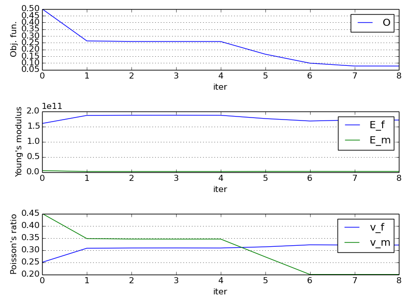
The resulting values of , , ,
can be found at the end of the script output:
>>> material optimization FINISHED <<<
material_opt_micro: terminated
optimized parameters: [1.71129526e+11 3.20844131e-01 2.33507829e+09 2.00000000e-01]
So that:
Note: The results may vary across SciPy versions and related libraries.