Linear Combination Boundary Conditions
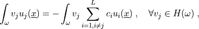
By linear combination boundary conditions (LCBCs) we mean conditions of the following type:
(1)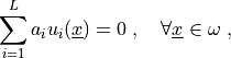
where  are given coefficients,
  are some
components of unknown fields evaluated point-wise in points
are some
components of unknown fields evaluated point-wise in points
 , and
, and  is a subset of the entire
domain
is a subset of the entire
domain  (e.g. a part of its boundary). Note that the
coefficients can also depend on
(e.g. a part of its boundary). Note that the
coefficients can also depend on  .
.
A typical example is the no penetration condition
 , where
  are the
velocity (or displacement) components, and
are the
velocity (or displacement) components, and  is the unit
normal outward to the domain boundary.
is the unit
normal outward to the domain boundary.
Enforcing LCBCs
There are several methods to enforce the conditions:
penalty method
substitution method
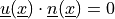
We use the substitution method, e.i. we choose  such that
 and substitute
(2)
into the equations. This is done, however, after the discretization by the finite element method, as explained below.
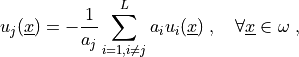
Let us denote  ( is fixed). Then
(3)
Weak Formulation
We multiply (3) by a test function  and
integrate the equation over to obtain
and
integrate the equation over to obtain
(4)
where  is some suitable function space (e.g. the same space
which
is some suitable function space (e.g. the same space
which  belongs to).
Finite Element Approximation
On a finite element  (facet or cell) we have
 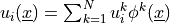 , where
  are the
local (element) base functions. Using the more compact matrix notation
are the
local (element) base functions. Using the more compact matrix notation
![\ub_i = [u_i^1, \dots, u_i^N]](_images/math/708247c676f7e8a7e538da6f4b84633479c01344.png) ,
, ![\vphib = [\vphib^1, \dots,
\vphib^N]^T](_images/math/f950c2875563a625176273728c930b6c5c6f8d28.png) we have
we have 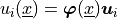 and similarly
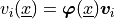 .
.
The relation (3), restricted to , can be
then written (we omit the arguments) as
(5)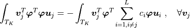
As (5) holds for any  , we have a linear
system to solve. After denoting the “mass” matrices
, we have a linear
system to solve. After denoting the “mass” matrices 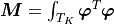 ,
, 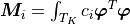 the linear system is
(6)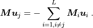
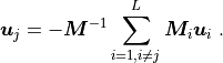
Then the individual coefficients  can be expressed as
(7)
Implementation
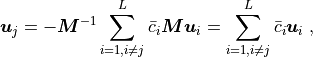
Above is the general treatment. The code uses its somewhat simplified
version described here. If the coefficients  are constant in
the element , i.e.
are constant in
the element , i.e.  for
for
 , we can readily see that
  . The relation (7) then reduces to
(8)
hence we can work with the individual components of the coefficient
vectors (= degrees of freedom) only, as the above relation means, that
 for
for  .
.