diffusion/time_poisson_explicit.py
Description
Transient Laplace equation.
The same example as time_poisson.py, but using the short syntax of keywords, and explicit time-stepping.
Find  for
for ![t \in [0, t_{\rm final}]](../_images/math/9f80775f131863202ea25954249a43c09294920c.png) such that:
such that:
r"""
Transient Laplace equation.
The same example as time_poisson.py, but using the short syntax of keywords,
and explicit time-stepping.
Find :math:`T(t)` for :math:`t \in [0, t_{\rm final}]` such that:
.. math::
\int_{\Omega} s \pdiff{T}{t}
+ \int_{\Omega} c \nabla s \cdot \nabla T
= 0
\;, \quad \forall s \;.
"""
from __future__ import absolute_import
from sfepy import data_dir
from sfepy.examples.diffusion.time_poisson import get_ic
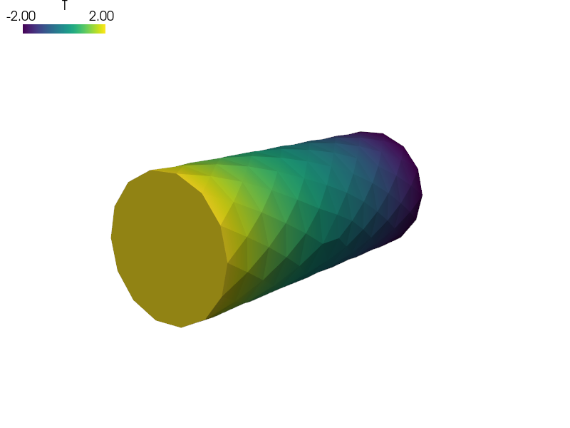
filename_mesh = data_dir + '/meshes/3d/cylinder.mesh'
materials = {
'coef' : ({'val' : 0.01},),
}
regions = {
'Omega' : 'all',
'Gamma_Left' : ('vertices in (x < 0.00001)', 'facet'),
'Gamma_Right' : ('vertices in (x > 0.099999)', 'facet'),
}
fields = {
'temperature' : ('real', 1, 'Omega', 1),
}
variables = {
'T' : ('unknown field', 'temperature', 0, 1),
's' : ('test field', 'temperature', 'T'),
}
ebcs = {
't1' : ('Gamma_Left', {'T.0' : 2.0}),
't2' : ('Gamma_Right', {'T.0' : -2.0}),
}
ics = {
'ic' : ('Omega', {'T.0' : 'get_ic'}),
}
functions = {
'get_ic' : (get_ic,),
}
integrals = {
'i' : 1,
}
equations = {
'Temperature' :
"""dw_dot.i.Omega( s, dT/dt )
+ dw_laplace.i.Omega( coef.val, s, T[-1] ) = 0"""
}
solvers = {
'ls' : ('ls.scipy_direct', {}),
'newton' : ('nls.newton', {
'i_max' : 1,
'is_linear' : True,
}),
'ts' : ('ts.simple', {
't0' : 0.0,
't1' : 0.07,
'dt' : 0.00002,
'n_step' : None,
'verbose' : 1,
}),
}
options = {
'ls' : 'ls',
'ts' : 'ts',
'save_times' : 100,
'output_format' : 'h5',
}